Phylogenetic trees

Learning Objectives This week, students will:

work with newick Files

learn to read phylogenies into R.

access and list the elements of a phylo object

understand the relationship between lists and the phylo class as data structures.

plot phylogenies with ape::plot.phylo() and ggtree::ggtree()

customize phylogenetic plots with ggtree::ggtree()

obtain phylogenetic data from the Open Tree of Life

get dated phylogenies using datelife

Practice Objectives

Exploring the structure of an object

Non Objectives

simulate phylogenies

plot phylogenies with ape

Day 1: Reading and plotting phylogenies

Setup your RStudio project (5 min)

🎗️ Structuring your files into a project is a best practice for good data science!
Open your RStudio project for the class; I called mine “fall-2022”.
Open a new Rmd file, name it “portal-phylogenies.Rmd”, and save it to your “documents” folder.

The newick format (10 min)

Download this phylogenetic tree of species from the Portal Project Teaching Database, by clicking on the link and saving it to your data-raw folder.
Open the file by clicking on its name on the Files tab of RStudio’s Plots pane. It should look like this:

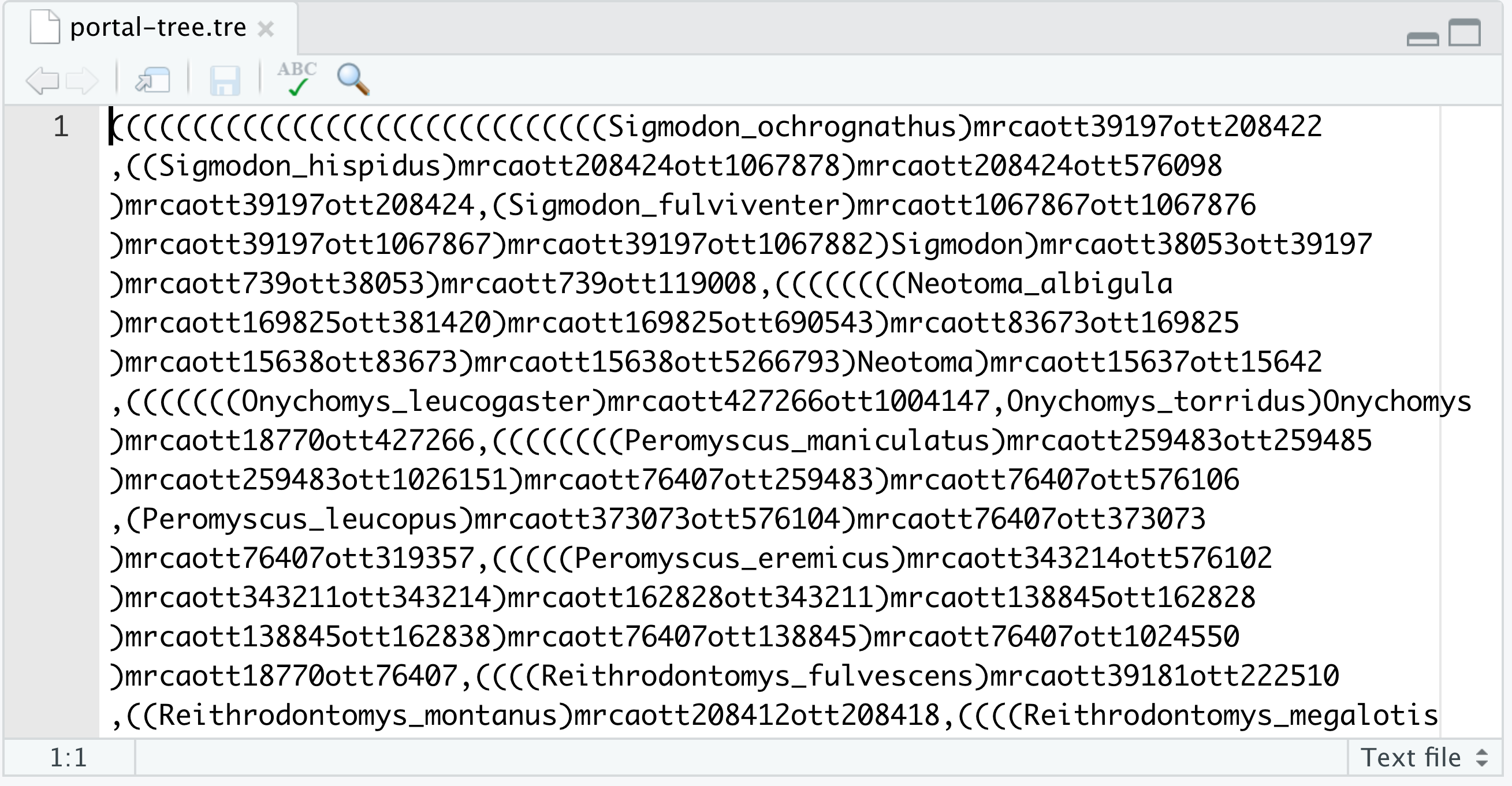
This is a newick file!
- It is a text file that represents a phylogenetic tree
- this format allows a computer to read the tree easily: it is in computer-readable form
- each pair of matched parenthesis ( ) represents an inner node
- character strings (names) within parentheses represent a tip
- a comma , separates nodes and tips, and represents a lineage
- the semicolon ; represents the end of the tree
⚠️ The existence of the newick format is very important because we can’t (yet) analyse data using a computer (either from tables or trees) if it is in image (png, jpg, pdf, etc.) format.

The package `ape` (5 min)

the name of the package ape is an acronym that stands for Analysis of Phylogenetics and Evolution
it was mainly developed for the analysis of molecular sequences
install.packages("ape")

Read a phylogeny into R (10 min)

read.tree() function from the package ape
Usage to read a phylogeny from a newick file in your computer:
- provide the path and file name
- 🎗️ Use relative paths!
```
ape::read.tree("relative/path/newick-file-name.tre")
```
Usage to read a phylogeny from a URL address:
- Provide the URL address as a character vector:
```
ape::read.tree("url.adress/newick-file-name.tre")
```
Example:
- Read into R the newick tree in the file “portal-tree.tre”
- create an object named portal_tree:
```
portal_tree <- read.tree(file = "../data-raw.portal-tree.tre")
```
- Read into R the newick tree from URL “http://ape-package.ird.fr/APER/APER2/primfive.tre”,
- To copy the URL, go to ape’s book website and copy the link to primfive.tre
- create an object named small_tree:
```
small_tree <- read.tree(file = "http://ape-package.ird.fr/APER/APER2/primfive.tre")
```

The `phylo` class structure (10 min)

Compare all outputs as applied to a data frame, such as surveys <- read.csv("../data-raw/surveys.csv")

Type the name of the objects you just created and look at the output
What information is printed to screen?
Use functions to explore the structure of the objects you just created:
- class(portal_tree), portal_tree is an object of class "phylo"
- length(tree), it has length 4
- names(tree), and it has names
- Just as with data frames, we can access the named elements of a "phylo" object using the dollar sign $
  - portal_tree$edge, class(portal_tree$edge)
  - portal_tree$Nnode,
  - portal_tree$tip.label
  - portal_tree$node.label
- str(tree), shows a summary of the elements of the "phylo" object
- typeof(tree), the "phylo" class is an object of type "list"
🎗️ classes and types are data structures that R uses to store/extract information
a "list" is a data type (or object type), that can hold one or more objects of different types.
the class "phylo" is a list that combines a matrix, a numeric vector of length one and two character vectors.
the "phylo" class provides R with all the information it needs to represent a phylogenetic tree

Plot a phylogeny with the package `ape` (5 min)

plot.phylo() function from the package ape:

plot.phylo(portal_tree)
plot.phylo(small_tree)

plotting phylogenies with ape requires a lot of customization.
we will not cover that in this course,

Installing the package `ggtree` (10 min)

ggtree is an extension of the ggplot2 package, developed specifically for phylogenetic tree visualization
The author has made available an extensive book with examples
ggtree is hosted in Bioconductor (not CRAN.
do length(available()) if you want to know the number of R packages available for installation, both from CRAN and Bioconductor
“CRAN hosts over 15000 packages and is the official repository for user contributed R packages. Bioconductor provides open source software oriented towards bioinformatics and hosts over 1800 R packages”, from An Introduction to R
Bioconductor Vs CRAN
The function install.packages() that we know well only workf for CRAN packages
To install an R package from Bioconductor, use the function install() from the package BiocManager:
1. Install BiocManager from CRAN with install.packages("BiocManager")
2. Then install ggtree from Bioconductor with BiocManager::install("ggtree")

Plot a phylogeny with the package `ggtree` (5 min)

The main function to visualize trees is also called ggtree():
```
ggtree(portal_tree)
```

It is a wrapper of:

ggplot(tree, aes(x, y)) +
geom_tree() +
theme_tree()

ggtree – as ggplot, uses the plus symbol + to add plotting layers.

Display a scale (5 min)

Use the function geom_treescale()
```
ggtree(portal_tree) +
geom_treescale()
```
how is the timescale calculated?

Access Branch lengths (5 min)

data in "edge.length" is used to plot the timescale in the small_tree visualization
how is the timescale calculated in trees with no "edge.length"?
Get branching times with branching.times()

Exercise 1: A scale for `small_tree` (10 min)

Plot the small tree of five species of primates and include a scale.
```
ggtree(small_tree) +
geom_treescale()
```
What is the difference in terms of data structure between the two trees?
- Trees differ in number of tips (43 vs 5)
```
length(portal_tree$tip.label)
length(small_tree$tip.label)
```
- They also differ in that small_tree has no node labels, but it has an "edge.length" element that portal_tree does not have.
- This is where branch length data is stored. Access it with branching.times(small_tree).

A mouse lemur (Primates)	A kangaroo rat (Rodentia)

Plot tip labels (5 min)

Use the function geom_tiplab()

the fontface = argument allows plotting species names in italics

ggtree(portal_tree) +
geom_tiplab(size = 3, color = "purple", fontface = 3) # or fontface = "italic"

If tip labels are truncated, give more plotting space with the function xlim()
- xlim() requires two numbers, specifying the start and end of the x axis.
- specifying an NA will let R choose the default limit for the axis:
```
... +
xlim(NA,20)
```

Exercise 2: Tip labels for `small_tree` (5 min)

Plot the small tree of five species of primates; include a scale, and tip labels.
Use the function branching_times() to set up an appropriate limit for the x axis, so tips are fully displayed (not truncated).

Day 2: Joining phylogenies to data tables

Setup your RStudio project (5 min)

🎗️ Structuring your files into a project is a best practice for good data science!
Open your RStudio project for the class; I called mine “fall-2022”.
Go to your “documents” folder and open the Rmd file for this topic; it should be named “portal-phylogenies.Rmd”.

Define a phylogenetic tree (10 min)

What is a phylogeny?
A phylogeny is a hypothesis of ancestor-descendant relationships (aka evolutionary relationships)/
We represent this hypothesis graphically in the form of a tree:

The main parts of a phylogenetic tree are:
- Tips, represent our observations; either a living species, a fossil, a sample of a virus, etc.
- Nodes, represent a hypothesis of common ancestry. That means, based on evidence, we think that two or more lineages share a common acestor some time in the past; or that two or more lineages descend from the same lineage and diverged from it some time in the past.
- Branches, represents a measure of amount of change that occured between lineages in a measure of time (commonly known as evolutionary distance).
  - branches by themselves cannot say in wich direction the change occurred.
- Root, is a special type of node, as it represents the common ancestor to all lineages in the tree.
  - The position of the root provides a direction of evolution.

Both of these phylogenetic trees shows the relationship of the three domains of life (Bacteria, Archaea, and Eukarya), but the (a) rooted tree attempts to identify when various species diverged from a common ancestor, while the (b) unrooted tree does not.

Caption from original Figure 20.1𝐴.1 of LibreTexts

Tree representation: layouts (5 min))

The argument layout = for the function ggtree().
It has several options: one of "rectangular", "dendrogram", "slanted", "ellipse", "roundrect", "fan", "circular", "inward_circular", "radial", "equal_angle", "daylight" or "ape".

ggtree(tr = portal_tree, layout = "roundrect")

ggtree(portal_tree, layout="slanted")
ggtree(portal_tree, layout="ellipse")
ggtree(portal_tree, layout="circular")
ggtree(portal_tree, layout="fan", open.angle=120)
ggtree(portal_tree, layout="fan", open.angle=15)
ggtree(portal_tree, layout="equal_angle")
ggtree(portal_tree, layout="daylight")

Subplots

It is possible to use facets as with ggplot()
We will use the package aplot
Install it from CRAN:
```
install.packages("aplot")
```

usage of function plot_list():

plot_list(plot1, plot2, tag_levels = "A")

Example with option tag_levels =

plot_list(ggtree(portal_tree, layout="circular"),
        ggtree(portal_tree, layout="fan", open.angle=15),
        tag_levels = "A")

Example with option labels =

plot_list(ggtree(portal_tree, layout="circular"),
        ggtree(portal_tree, layout="fan", open.angle=15),
        labels = c("Circular", "Fan"))

Exercise: Tree representation.

Try the following layouts on your tree of Portal species:

ggtree(portal_tree, layout="ape")
ggtree(portal_tree, layout="rectangular")
ggtree(portal_tree, layout="roundrect")
ggtree(portal_tree, layout="slanted")
ggtree(portal_tree, layout="ellipse")
ggtree(portal_tree, layout="dendogram")
ggtree(portal_tree, layout="circular")
ggtree(portal_tree, layout="radial")
ggtree(portal_tree, layout="fan", open.angle = 90)
ggtree(portal_tree, layout="equal_angle")
ggtree(portal_tree, layout="daylight")
ggtree(portal_tree, layout="unrooted")

Create a plot containing a subplot for each one of them.
As title for each subplot, indicate if the tree representation is rooted or unrooted.
Which layout options display the same tree visualization?

Difference between phylogeny and taxonomy (5 min)

What is taxonomy?
The science of description, identification, nomenclature, and classification of organisms.

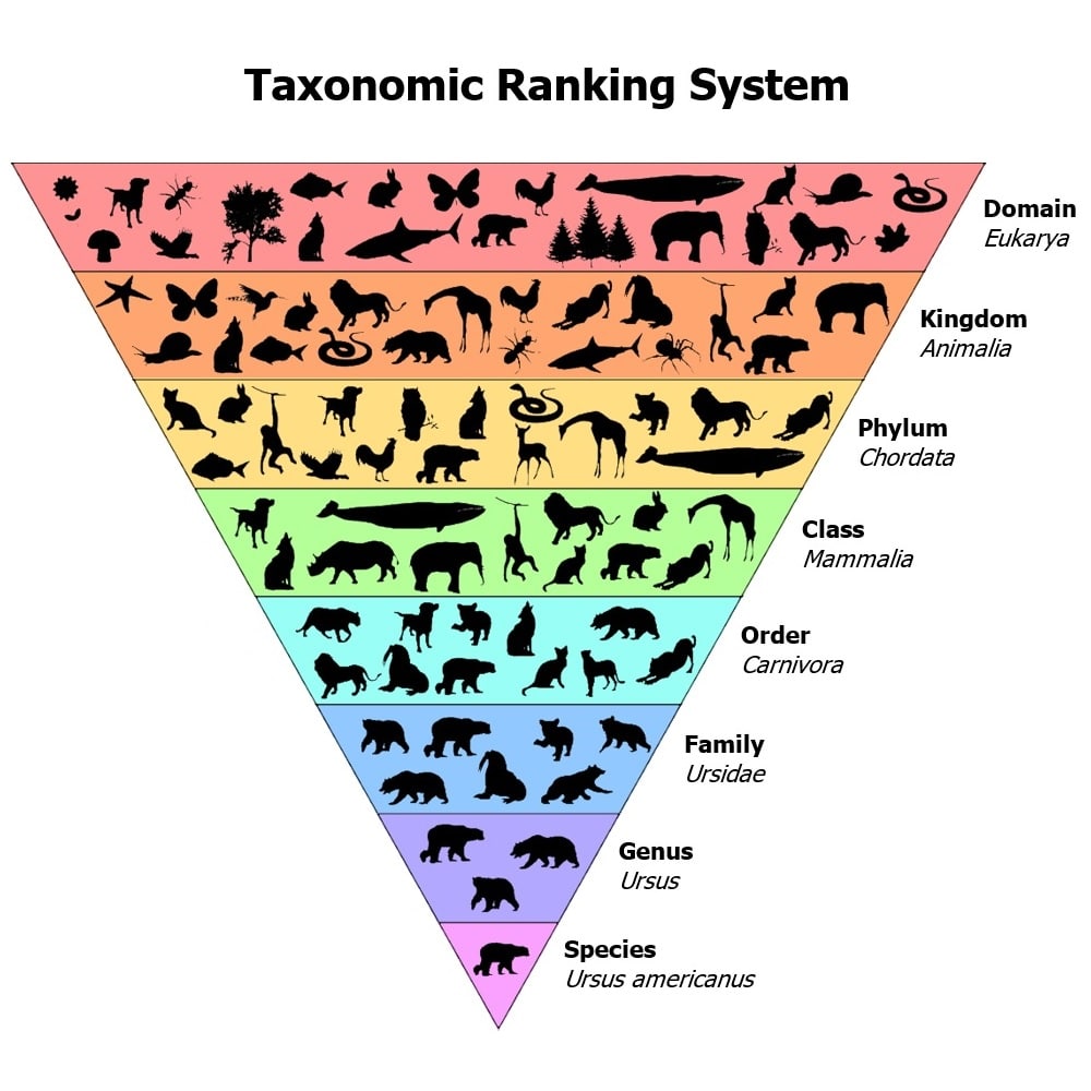
In a broad sense, taxonomy is the method used for organizing similar content into relevant groups. To put it even more broadly, taxonomy is how we classify things. From its conception, taxonomies have played an important role in biological science, where it has been largely used to organize the animal kingdom. Think of mammals vs. birds vs. reptiles and all the details in between: within the mammals group, we have cats, whales, apes, etc.; as we move further down the line, we have different species of apes such as gorilla, chimpanzees, etc. If you can visualize this as a tree of sorts, you’re already on the way to understanding what a taxonomy is at its basic level.

Text from Taxonomy management 101.

Connecting a phylogeny with data from a table

Preparation:
1. Download a data table of the species from the Portal Data base that inlcudes taxonomy
2. Save it in your data-raw folder.
3. Read it into R with read.csv(), and assign it to an object called taxonomy.

To join a tree and a data table, we will use the _join() functions that we used previously to join tables
How do they work? Example with surveys and species.
To link a tree and a data table, the tree is the first argument and the table is second:
```
full_join(portal_tree, taxonomy_matched, by= "label")
```
What is the structure of the object?
Attention! doing a full join does not work down the analysis flow, we need a left join to drop non matches
```
tree_table <- left_join(portal_tree, taxonomy, by = "label")
```
We can still plot our tree normally with ggtree(tree_table)

But now we can use aesthetics to plor our tip labels with certain group by color:

ggtree(tree, aes(color = taxa, fontface = "italic")) + # it freezes if there are any unmatched or NA labels in data table!!!
xlim(0, 20) +
geom_tiplab()

Exercise: A taxonomy table for `small_tree`

Find the appropriate scientific group labels for each genus in small_tree using this tree as guide.
Create a data frame with 3 columns:
- a "label" column with the names of the tip labels of small_tree. Tip: extract the element "tip.label" from your phylo object to get a vector of tip labels that you can then join to the other vectors to create a data frame.
- a "taxa" column with the scientific names of the group that each genus belongs to.
- a "common_name" column with the common names of the group that each genus belongs to. Tip: use the function c() to create the vectors that will be columns "taxa" and "common_name"
Join your tree and your table using left_join().
Create two different tree plots using taxa and common name to color the tips of the tree.

Day 3:

Setup your RStudio project (5 min)

🎗️ Structuring your files into a project is a best practice for good data science!
Open your RStudio project for the class; I called mine “fall-2022”.
Go to your “documents” folder and open the Rmd file for this topic; it should be named “portal-phylogenies.Rmd”.

Review: Creating data Tables (40 min)

Questions from homework?
Updating the portal tree and taxonomy table
Joining tree and data

Intro to the data set (10 min)

Load and install the necessary packages:

library(ggimage)
library(ggtree)
install.packages("TDbook")
library(TDbook)
library(tidytree)

use function data() to load a tree and data table data from package TDbook:
- tree_boots,
- df_tip_data,
- df_inode_data
```
data("tree_boots", "df_tip_data", "df_inode_data")
```

Plot Data to tree tips (10 min)

Change the "newick_label" column name of the data tables to "table":
```
colnames(df_tip_data)[1] <- "label"
```

Use left_join() to join data table and tree

tree_joined <- left_join(tree_boots, df_tip_data, by = "label") # only works with by = "label", not with "Newick_label"
tree_joined

add data on weight to tips with geom_tippoint()

ggtree(tree_joined) +
geom_tippoint(aes(shape = "circle",
                  color = trophic_habit,
                  size = mass_in_kg))

Exercise: Mapping weight data from surveys CSV table to the portal tree (10 min)

Get the average weight and hindfoot length per species.
Create a new data frame that contains the taxonomy data plus the averaged data per species that you got on last question.
Create two plots with data on the tips, one with the average weight and the other with average hindfoot length. Make sure to also add tip labels, formatted in italics.

Day 4

Review: Joining trees and data

Questions from homework?

Setup your RStudio project

🎗️ Structuring your files into a project is a best practice for good data science!
Open your RStudio project for the class; I called mine “fall-2022”.
Go to your “documents” folder and open a new Rmd file for this topic; it should be named “portal-phylogenies-day4.Rmd”.

Load and the necessary packages:

library(ggimage)
library(ggtree)
library(TDbook)
library(tidytree)

Load the data:
```
data("tree_boots", "df_tip_data", "df_inode_data")
```
Exercise: Explore the data
1. What is the class of tree_boots? How many elements does it have?
2. What is the class of df_tip_data? How many rows does it have? Compare this to the length of tip labels in tree_boots
3. What is the class of df_inode_data? How many rows does it have? Compare this to the length of node labels in tree_boots
4. Are the column names in the two data frame objects the same or different?

Access elements of a `"treedata"` object

Join the tree_boots tree with df_tip_data and create an object called tree_joined
Explore the object
- Type its names and hit return
- Use the following functions
```
str(tree_joined)
class(tree_joined)
length(tree_joined)
```
Use the @ to access firt elements, then $. Look at the names of the element ExtraInfo. These are the column names of the data table.

Plot node labels from a data table

Introduction:
- So far we have plotted things on tips of the tree.
- To plot node data, we need to join the tree and the data table with node data.
  - The df_inode_data object has data about the nodes of the tree.
To join a data table and a tree, we must check the column names of the data table. The column name that contains the tip labels mus be named "label":
```
colnames(df_inode_data)
colnames(df_inode_data)[1] <- "label"
```
We can join this data table in two ways:
- We can join this data table to the tree directly (portal_tree)
- Or, in the same way we join multiple tables, we can join a new table to our treedata object:
```
tree_data <- left_join(tree_joined, df_inode_data, by = "label")
tree_data
```
Explore the names of @ExtraInfo
Pay attention to the names of the columns from df_inode_data.

We will use these names to add node labels to the tree.

ggtree(tree_data) +
geom_label(aes(label = vernacularName.y, fill = vernacularName.y))

Exercise: Node labels for the Portal tree

Add node labels to your two tree plots with average weight and hindfoot length. Use the column "taxa" both as label and fill color.

Plot node labels from a tree

The function geom_nodelab() adds names to nodes of a tree that are stored in the $node.label element:
```
ggtree(tree_boots) +
geom_nodelab(size = 3, color = "blue")
```

Exercise: More node labels for the Portal tree

Add node labels to the portal tree using data from the $node.label element.

Getting trees from an Open data base

How do we construct phylogenetic trees?
How long does it take?
Open Science and Data Science
The Open Tree of Life project
the rotl package.
the Open Tree of Life Taxonomy
matching names to OTT
Getting a tree from Open Tree using R

Data Science Research in Biology - Fall 2022

Day 1: Reading and plotting phylogenies

Setup your RStudio project (5 min)

The newick format (10 min)

The package ape (5 min)

Read a phylogeny into R (10 min)

The phylo class structure (10 min)

Plot a phylogeny with the package ape (5 min)

Installing the package ggtree (10 min)

Plot a phylogeny with the package ggtree (5 min)

Display a scale (5 min)

Access Branch lengths (5 min)

Exercise 1: A scale for small_tree (10 min)

Plot tip labels (5 min)

Exercise 2: Tip labels for small_tree (5 min)

Day 2: Joining phylogenies to data tables

Setup your RStudio project (5 min)

Define a phylogenetic tree (10 min)

Tree representation: layouts (5 min))

Subplots

Exercise: Tree representation.

Difference between phylogeny and taxonomy (5 min)

Connecting a phylogeny with data from a table

Exercise: A taxonomy table for small_tree

Day 3:

Setup your RStudio project (5 min)

Review: Creating data Tables (40 min)

Intro to the data set (10 min)

Plot Data to tree tips (10 min)

Exercise: Mapping weight data from surveys CSV table to the portal tree (10 min)

Day 4

Review: Joining trees and data

Setup your RStudio project

Exercise: Explore the data

Access elements of a "treedata" object

Plot node labels from a data table

Exercise: Node labels for the Portal tree

Plot node labels from a tree

Exercise: More node labels for the Portal tree

Getting trees from an Open data base

Data Science Research in Biology -
Fall 2022

The package `ape` (5 min)

The `phylo` class structure (10 min)

Plot a phylogeny with the package `ape` (5 min)

Installing the package `ggtree` (10 min)

Plot a phylogeny with the package `ggtree` (5 min)

Exercise 1: A scale for `small_tree` (10 min)

Exercise 2: Tip labels for `small_tree` (5 min)

Exercise: A taxonomy table for `small_tree`

Access elements of a `"treedata"` object