7. Summarizing branch length information

Overview

Teaching: 5 min
Exercises: 5 min

Questions

• How do I summarize information from different source chronograms?

• How do I choose a preferred source chronogram?

Objectives

• Understanding the depth of uncertainty around age estimates.

Now that we have a collection of chronograms containing our taxa of interest, we can go on to summarize the information in them.

There is no consensus on the best way to do this.

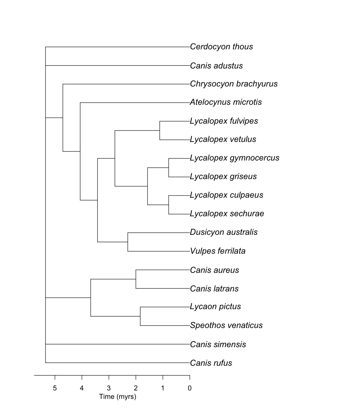
We have implemented two ways of summarizing information from several chronograms into a single one. The fastest one is using the median of node ages for each node with available information, and then evenly distributing ages across nodes.

canis_phylo_median <-  datelife::summarize_datelife_result(canis_dr, summary_format = "phylo_median")

Check that we actually went from a list of matrices to a tree with branch lengths:

canis_phylo_median

Phylogenetic tree with 18 tips and 13 internal nodes.

Tip labels:
	Canis_rufus, Canis_simensis, Speothos_venaticus, Lycaon_pictus, Canis_latrans, Canis_aureus, ...
Node labels:
	n1, n2, n3, n4, n5, n6, ...

Unrooted; includes branch lengths.

Good. Now we can plot our chronogram!

ape::plot.phylo(canis_phylo_median, cex = 1.2)
# Add the time axis:
ape::axisPhylo()
# And a little hack to add the axis name:
graphics::mtext("Time (myrs)", side = 1, line = 2, at = max(get("last_plot.phylo",envir = .PlotPhyloEnv)$xx) * 0.5)

Challenge! Get the other type of summary chronogram

Hint: Explore options from the argument summary_format in the function summarize_datelife_result()

Solution

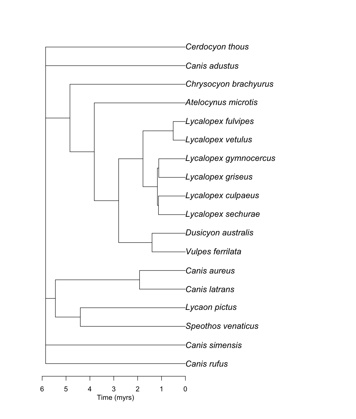
canis_phylo_sdm <-  datelife::summarize_datelife_result(canis_dr, summary_format = "phylo_sdm")

canis_phylo_sdm

Phylogenetic tree with 18 tips and 13 internal nodes.

Tip labels:
	Canis_rufus, Canis_simensis, Speothos_venaticus, Lycaon_pictus, Canis_latrans, Canis_aureus, ...
Node labels:
	n1, n2, n3, n4, n5, n6, ...

Unrooted; includes branch lengths.

ape::plot.phylo(canis_phylo_sdm, cex = 1.2)
ape::axisPhylo()
graphics::mtext("Time (myrs)", side = 1, line = 2, at = max(get("last_plot.phylo",envir = .PlotPhyloEnv)$xx) * 0.5)

As you can note, the SDM sumary chronogram is slightly older than the median summary chronogram!

Finally, give it a try on the web browser of datelife, too. You can do the same things using a graphical user interface. It is fun!

Key Points

• Source chronograms have a wide range of variation in age estimates.